Abstract
We establish a rigorous mathematical framework for the spontaneous formation of stable structures through the universal principle of energy minimization in multi-interaction systems. Within this formulation, each subsystem contributes to a collective energy function E(x) composed of bounded, weakly nonlinear interaction terms. By proving the strictly positive definiteness of the Hessian and the existence of a unique critical point Q_c satisfying ∇E(Q_c)=0, we demonstrate that the system converges globally to this equilibrium via gradient-flow dynamics. Local and global stability are verified analytically through Lyapunov functions and LaSalle’s Invariance Principle under the assumptions of uniform strong convexity and coercivity. The resulting equilibrium represents a spontaneously formed structure that minimizes the total energy of the interacting fields. Extending beyond reaction–diffusion theory, the proposed framework unifies the energetic mechanisms of self-organization observed across physics, chemistry, and biology. As an illustrative application, the spontaneous assembly of lipid bilayers is interpreted as the natural descent toward a unique global energy minimum, providing a quantitative bridge between thermodynamic stability and dynamic self-organization. This study thus establishes energy minimization as a universal law governing the emergence, persistence, and stability of complex structures in nonlinear systems.
Keywords
Morphogenesis, Reaction-diffusion systems, Pattern formation, Self-organization, Interacting forces
1. Introduction
Life abounds with countless forms and patterns that characterize the immense diversity of organisms around us. The complexity of these patterns—whether in the morphology of individual organisms or within entire ecosystems—has intrigued scientists for decades. Understanding how such biological forms and patterns arise has long been a central question in developmental biology. In 1952, Alan Turing established the mathematical foundation of morphogenesis in his seminal work “The Chemical Basis of Morphogenesis” [1]. He introduced the reaction–diffusion model, proposing that spatial concentration differences among interacting chemical species could spontaneously give rise to ordered structures such as stripes or spots. This concept offered an elegant explanation for a wide range of natural patterning phenomena. Building on Turing’s insight, Gierer and Meinhardt [2] formulated the local-activation–lateral-inhibition model, clarifying the self-organizing logic of early embryonic patterning. Later, Oster and Murray [3] extended these frameworks by incorporating mechanical forces into morphogenetic theory, thereby linking chemical and physical interactions within tissues. This integration represented a major step toward realistic, multiscale models of biological form. In the late 20th and early 21st centuries, Kondo and Miura [4] demonstrated the applicability of reaction–diffusion principles to living systems, notably in pigment patterning of fish skin. Further experimental studies on zebrafish confirmed these models in vivo [5,6]. These works solidified Turing patterns as a core paradigm in developmental biology. Advances in computation have since enabled quantitative simulations of morphogenesis. Numerical methods and high-performance modeling have expanded the predictive capability of reaction–diffusion systems, revealing complex pattern transitions and multistable states [7]. At the same time, theoretical reviews such as Kondo [8] highlighted that real biological pattern formation often exceeds the scope of traditional two-component systems, requiring integration of genetic, mechanical, and environmental factors. While Turing’s framework successfully explains spontaneous symmetry breaking in simple chemical systems, real biological organization typically arises from multiple simultaneously interacting forces—chemical, mechanical, and dynamical. Examples include mechanical feedback between cells and extracellular matrices, chemomechanical coupling in tissue morphogenesis, and the influence of stochastic fluctuations or “biological noise” on developmental trajectories [9–11]. These phenomena imply that structure formation results not from a single reaction–diffusion pair but from the balance among diverse competing fields. The present study therefore advances a general energetic-minimization framework that transcends reaction–diffusion theory. Here, structural formation is viewed as an emergent outcome of energy minimization under multiple interacting constraints. Each subsystem—or “force field”—contributes to an effective potential, and the equilibrium configuration corresponds to the global minimum of this collective energy landscape. Before the formal mathematical development, the system’s essence can be intuitively understood through a physical analogy: a ball rolling down a complex energy surface. Each coordinate represents a possible configuration, while the slope corresponds to the gradient of potential energy. The ball naturally moves downhill until it reaches the lowest valley—where energy is minimized and the configuration becomes stable. The basin of attraction delineates the range of initial states that converge to this equilibrium. This image captures the core principle of the present theory: spontaneous structure formation arises inevitably from the minimization of total energy across interacting forces. Building on the above context, this paper provides a two-stage theoretical proof and a unified physical interpretation of self-organization driven by energetic minimization:
- Linear regime – local stability: Chapter 2 formulates a system governed by linear interactions and a convex quadratic energy function. It proves that the Hessian matrix is strictly positive definite, ensuring convexity and thus local stability of the equilibrium x0. Using a Lyapunov function, it demonstrates monotonic convergence of all trajectories within the local basin toward x0.
- Nonlinear regime – global convergence: Chapter 3 generalizes the analysis to a nonlinear energy landscape, incorporating higher-order coupling terms. Through Gerschgorin’s circle theorem [12] and LaSalle’s invariance principle [13], it shows that, under specified constraints, the system retains global convexity and every trajectory converges uniquely to the global energy minimum x0.
- Unified framework and implication: Together, these results establish a universal principle: stable structure formation is a natural consequence of energy minimization in multi-interaction systems. This principle applies equally to physical, chemical, and biological morphogenesis—linking molecular self-assembly, cellular patterning, and large-scale developmental organization within a single theoretical landscape.
2. Proposition and Its Proof (Linear Case)
This section rigorously demonstrates the spontaneous formation of stable structures in a system of multiple linear interactions governed by an energy minimization principle. By analyzing the convexity of the energy functional and the strictly positive definiteness of its Hessian, we establish both the existence and stability of an equilibrium point. The proof is structured around classical results from convex optimization and Lyapunov stability theory [14,15].
2.1 Assumptions for the proof
1) Linear interaction functions: Let Ω⊂Rnbe the state space of the system, where m independent linear interactions Ai(x) are defined:
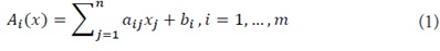
where aij,bi∈R are constants. Each Ai(x) is linear, continuously differentiable, and Lipschitz continuous in x.
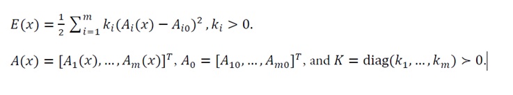
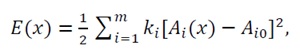
2) Energy function: Define the total energy function E(x) as:
 (2)
(2)
Let A(x)=[A1(x),…,Am(x)]T, A0=[A10,…,Am0]T, and K=diag(k1,…,km)>0.
Then E(x) can be written compactly as:
 (3)
(3)
This quadratic form guarantees that E(x) is twice continuously differentiable and convex.
3) Gradient and hessian: Since A(x)=Ax+b, where A=[aij],
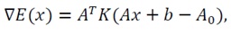 (4)
(4)
 (5)
(5)
The Hessian H is constant, symmetric, and positive semi-definite. If Ahas full column rank (rank(A)=n), then H>0, ensuring strict convexity and a unique global minimizer x0.
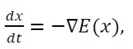
4) System dynamics: The temporal evolution of the system follows the gradient flow:
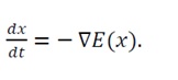 (6)
(6)
This differential equation describes a gradient descent flow representing a physical relaxation toward energy minimization.
5) Lyapunov function: Define the Lyapunov candidate function:
 (7)
(7)
where x0satisfies ∇E(x0)=0.
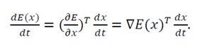
The time derivative is:
 (8)
(8)
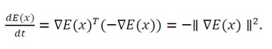
Thus, V(x) is strictly positive definite, and V(x) is negative semi-definite.
Under strict convexity (H>0), V(x)→0 only at x0, establishing global asymptotic stability.
2.2 Proof
Proposition: If there exists x0∈Ω such that ∇E(x0)=0 and the Hessian H=ATKA is strictly positive definite, then the system converges globally to x0, and a spontaneous stable structure is formed at this equilibrium.
Step 1: Stationary point condition
At equilibrium,
 (9)
(9)
Since H=ATKA>0, this critical point is the unique global minimum of E(x).
For any perturbation δx=x-x0:
 (10)
(10)
Step 2: Energy variation
Using the second-order Taylor expansion:
 (11)
(11)
As H>0, E(x) increases quadratically with IIδxII; hence the equilibrium x0 is locally (and globally) stable.
Step 3: Eigen-decomposition interpretation
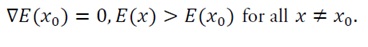
Let H=QΛQT, where Λ=diag(λ1,…,λn)with λi>0. Here, Qc denotes the equilibrium (critical) point of the system, defined by the stationary condition ∇E(Qc)=0. The deviation from equilibrium is defined as δx=x-Qc; at the equilibrium itself, δx = 0.
Thus, the condition x=Qc (or equivalently δx=0) identifies the spontaneously formed stable structure.
In the eigenbasis coordinates corresponding to Q, we have
 (12)
(12)
Hence, all perturbations increase the energy, confirming convexity and stability of the equilibrium.
Step 4: Dynamic convergence
The system follows the gradient flow:
 (13)
(13)
The solution converges exponentially to x0, since the linearized dynamics near equilibrium are:
 (14)
(14)
Step 5: Lyapunov stability
 . (15)
Because H=ATKA>0, the right-hand side is strictly negative for all x≠x0, confirming that the equilibrium is globally asymptotically stable. Since E(x)is radially unbounded (i.e., E(x)→∞as IIxII→∞), all trajectories remain bounded, and LaSalle’s invariance principle ensures global asymptotic convergence to x0.
2.3 Interpretation and summary
This proof demonstrates that, in a linear multi-interaction system, the energy landscape E(x)=12(Ax+b-A0)TK(Ax+b-A0) is strictly convex when Ais full-rank and K>0. Consequently, the system possesses a unique global energy minimum x0that represents a spontaneously stable configuration. The gradient-flow dynamics guarantee monotonic energy descent, while the Lyapunov framework rigorously ensures global stability.
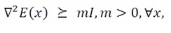
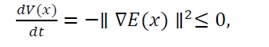
Figure 1 summarizes the schematic representation:
– Linear interaction functions Ai(x) define the system.
– The energy function E(x) forms a convex quadratic potential.
– The Hessian H=ATKA is strictly positive definite.
– Gradient dynamics x=-∇E(x) ensure monotonic energy descent.
– The Lyapunov function V(x)=E(x)-E(x0) confirms convergence to the unique equilibrium x0.
Collectively, these findings demonstrate that spontaneous structural stabilization naturally emerges from energy minimization under coupled linear interactions.

Figure 1. Schematic representation of energy-minimizing structural formation. Conceptual illustration showing how local interactions among subsystems collectively drive the system toward a globally minimized energy configuration. Arrows indicate gradient-flow directions leading to the equilibrium state x0 .
.
3. Proposition and Its Proof (Nonlinear Case)
The linear model presented in Chapter 2 provides a foundational understanding of stable structure formation. However, many real-world systems exhibit complex dynamics influenced by nonlinear interactions. To address this, this chapter extends the theoretical framework to incorporate nonlinear energy functions, aiming to establish global stability and convergence to a unique stable structure. The primary challenge lies in rigorously demonstrating the strictly positive definiteness of the Hessian matrix and, consequently, the strict convexity of the energy function in the presence of these nonlinear terms. To achieve this, the existence of a unique global energy minimum is targeted. For this minimum point to exist and yield a stable structure, two primary conditions must be satisfied: First Condition (Critical Point): At x_0, the gradient of the energy function must vanish, i.e., ∇E(x_0)=0. Second Condition (Strictly positive definiteness of the Hessian Matrix): The Hessian matrix H(x_0)at the energy minimum must be strictly positive definite. This condition ensures that the energy minimum point is locally stable [2,16]. Furthermore, by introducing a Lyapunov function and employing LaSalle’s Invariance Principle, this chapter establishes that all trajectories of the system, regardless of initial conditions, converge to the unique equilibrium corresponding to the global energy minimum, provided that Assumptions (U) (Uniform Strong Convexity) and (C) (Coercivity) hold. The influence of nonlinear terms on the stability of the system is also examined, demonstrating that their contribution, under specific constraints, is primarily limited to higher-order effects and does not compromise overall stability. This expanded framework provides a comprehensive proof of global stability for systems with nonlinear interactions, complementing and extending the insights gained in the previous chapter.
3.1 Definition of the energy function
We extend the interaction terms A_i (x) to include quadratic nonlinearities. While more complex nonlinearities exist, focusing on these quadratic terms allows for analytical tractability while still capturing essential aspects of self-regulatory or self-enhancing/inhibiting effects within components.
Assumption 6: The nonlinear interaction terms A_i (x)are given by:
 (16)
(16)
where a_ij and b_i are constants, and c_ijare coefficients of the nonlinear terms. We specifically assume that c_ij=0 for i≠j, meaning only quadratic terms involving a single variable are present (i.e., c_ii x_i^2). This simplifying assumption is valid in systems where higher-order interactions primarily manifest as self-regulatory or self-enhancing/inhibiting effects, rather than complex cross-component feedback loops. It allows for a clearer analytical treatment of the influence of individual component nonlinearities on the overall system stability. Future work will explore more general forms of cross-term nonlinearities. The proposed nonlinear energy function E(x) is defined consistently with the linear case:
 (17)
(17)
where k_i>0are positive constants that adjust the contribution of each interaction A_i (x), and A_i0 represents a reference value that provides the reference position for the system to achieve its energy minimum [13–15].
3.2 Verification of the strictly positive definiteness of the hessian matrix
To establish the stable structure of the system, it is necessary to demonstrate that the minimum point x_0 of the energy function E(x) is a stable equilibrium point, meaning that the energy increases in the vicinity of x_0. This also implies the strict convexity of E(x), which is crucial for guaranteeing a unique global minimum. To verify this, we construct the Hessian matrix H(x) of the energy function E(x) and prove that this matrix is strictly positive definite:
 (18)
(18)
The Hessian matrix represents the curvature of the energy function. If the Hessian matrix H(x) is strictly positive definite for all x in the domain of interest (meaning that all its eigenvalues are positive), then the energy function E(x) is strictly convex. A strictly convex function has a unique global minimum, and energy increases in its vicinity, guaranteeing a stable structure.
Footnote: Note 1: The indices c_ij, c_ik, and c_ii refer to the same class of nonlinear self-interaction coefficients. Under the simplifying assumption c_ij=0 for i≠j, only diagonal terms c_ii remain effective. Therefore, c_ik appears in derivative expressions for mathematical generality, while physically it represents the self-nonlinearity coefficient c_ii.
3.2.1 Calculation of the hessian matrix of the energy function: The energy function is given by Eq. (16). The first-order partial derivative with respect to x_k is
 (19)
(19)
and under the assumption c_ij=0 for i≠j(i.e., only self-quadratic terms are present), we have
 (20)
(20)
 (21)
(21)
 (22)
(22)
The diagonal components are given by
 (23)
(23)
Since δ_ik=1 only when i=k, this may be expanded explicitly as

To guarantee strictly positive definiteness via a verifiable sufficient condition, we impose strict diagonal dominance (together with symmetry) rather than comparing only the two diagonal terms:
Condition 7 (Strict diagonal dominance for a symmetric Hessian)
For all xand all k,
 (24)
(24)
Since H(x)is real and symmetric by construction, condition (24) ensures H(x)?0 (Levy–Desplanques theorem), guaranteeing local strong convexity around the point of interest.
The off-diagonal components are given by
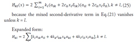 (25)
(25)
Remark
Eqs (23)–(25) provide all Hessian entries in closed form with correct index handling. Condition (24) serves as a sufficient (though not necessary) test for strictly positive definiteness; it improves upon prior diagonal-only criteria by directly constraining the entire symmetric matrix through a holistic, structure-compatible formulation.
Remark (Scope and limitation of nonlinearity)
In the present formulation, the nonlinear interaction terms are restricted to self-regulatory components, c_ij=0 for i≠j. This assumption ensures analytical tractability and preserves the diagonal-dominant structure of the Hessian matrix, which in turn guarantees convexity and a unique global minimizer of the energy function. Physically, this corresponds to systems in which nonlinear effects act primarily as self-stabilizing or self-inhibiting mechanisms within individual subsystems rather than as cross-couplings between them. Nevertheless, many real physical, chemical, and biological systems exhibit cooperative or competitive cross-interactions (c_ij≠0) that may generate richer dynamical behaviors such as multistability or pattern bifurcations. Extending the present framework to incorporate these cross-nonlinearities represents a natural and important direction for future work. Such an extension would generalize the convexity conditions derived here to block-structured Hessians and allow the theory to describe a broader class of self-organizing systems beyond purely self-regulatory dynamics.
Footnote.
Note 2: Here, c_ii denotes the self-nonlinearity coefficient of component i, and δ_ik (Kronecker delta) enforces that only terms with i=k contribute to the quadratic curvature. This formulation is equivalent to using c_ik with the convention c_ik=0 for i≠k, ensuring full consistency across derivative definitions and Hessian structure.
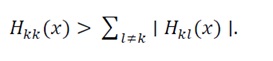
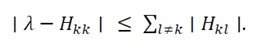
3.2.2 Verification of strictly positive definiteness using gershgorin’s circle theorem: To confirm the strictly positive definiteness of the Hessian matrix H(x), we bound its eigenvalues using Gershgorin’s Circle Theorem. For each diagonal entry H_kk, all eigenvalues λ of H(x) lie within the disk
 (26)
(26)
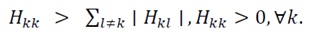
For a real symmetric matrix such as H(x)=H(x)^T, all eigenvalues are real, and these disks degenerate into intervals on the real axis. If every interval lies entirely in the positive half-line, then all eigenvalues are positive and H(x) is strictly positive definite. A sufficient condition ensuring this situation is strict diagonal dominance together with positive diagonals:
 (27)
(27)
Eq. (27) guarantees that every Gershgorin interval is contained in (0,∞), hence H(x)?0 and the energy landscape is locally convex around the point of interest. (This condition coincides with Condition 7 in Section 3.2.1.) While Gershgorin’s circle theorem provides a convenient and intuitive sufficient condition for strictly positive definiteness based on diagonal dominance, it is not a necessary one. A more rigorous and complete verification can be achieved using Sylvester’s criterion, which requires that all leading principal minors of the Hessian matrix be positive. In this study, Gershgorin’s theorem was adopted for its analytical transparency and geometric interpretability; however, for numerical analysis or applications to more complex, high-dimensional systems, it is recommended to employ Sylvester’s criterion in parallel to ensure comprehensive validation of strictly positive definiteness. It must be emphasized that diagonal dominance is a sufficient but not necessary criterion for strictly positive definiteness. Thus, the convexity certified by (27) is local to the subset of the state space where the inequality holds. To guarantee global strict convexity, we impose Uniform Strong Convexity:
 (28)
(28)
which in particular implies coercivity, E(x)→∞ as ?x?→∞. Under Assumption (U), the energy function E(x) possesses a unique global minimizer x_0. Within the admissible range of the state variables, Condition 7 and the diagonal-dominance relation ensure that diagonal curvature terms dominate cross-couplings—a physically intuitive scenario in which self-stabilizing effects outweigh mutual interactions. Hence, in the region where (27) holds, H(x) is strictly positive definite and E(x) is locally strongly convex; if in addition (U) holds, this convexity extends globally and the energy-minimizing equilibrium is unique.
Illustration (consistent with Section 3.2.1).
A representative diagonal element can be written as H_kk (x)=2∑_(i=1)^m??k_i [(a_ik+2c_ii " " x_i " " δ_ik )^2+(A_i (x)-A_i0)" " 2c_ii " " δ_ik]?. Since k_i>0, positivity is maintained provided (a_kk+2c_kk x_k)≠0over the physically relevant range of x_k. For example, if k_1=1, x_k∈[-1,1], and a_1k=1, then restricting c_11∈(-0.5,0.5) ensures H_kk>0 for all x_k. Therefore, Condition 7 limits the nonlinear self-coefficients c_iiso that quadratic nonlinearities remain sufficiently weak to preserve the positive curvature induced by linear interactions—preventing multistability or oscillations and ensuring convergence to a unique, stable equilibrium.
Footnote:
Note.3:c_ii denotes the self-nonlinearity coefficient of component i. The Kronecker delta δ_ik enforces that only terms with i=kcontribute to the quadratic curvature; this is equivalent to writing c_ikwith the convention c_ik=0 for i≠k.
3.3 Lyapunov function and global convergence analysis
This section rigorously establishes the global convergence of the nonlinear dynamical system x ?=-∇E(x), by employing a Lyapunov-based framework in conjunction with LaSalle’s Invariance Principle. Under the dual assumptions of Uniform Strong Convexity (U) and Coercivity (C), it is demonstrated that all trajectories asymptotically converge to a unique equilibrium x_0, which corresponds to the global minimum of the energy functional E(x).
Preliminaries for laSalle’s analysis
To formalize the argument, we define the following sets and relations that form the foundation of LaSalle’s invariance framework:
 (29)
(29)
 (30)
(30)
 (31)
(31)
These definitions bridge the convexity conditions introduced in Section 3.2 ((26)–(28)) with the convergence formulation presented here, ensuring logical and numerical continuity throughout the theoretical development.
3.3.1 Definition and strictly positive definiteness of the lyapunov function: To rigorously analyze the convergence behavior of the system, we define the Lyapunov function V(x) in terms of the energy function E(x) as:
 (32)
(32)
where E(x_0) denotes the minimum value of E(x) attained at the unique equilibrium point x_0. As demonstrated in Section 3.2, the energy function E(x) is locally strongly convex (and globally strongly convex under Assumption (U)), ensuring that x_0 uniquely satisfies
Thus, V(x) measures the “energy distance” from any state x to the equilibrium x_0, serving as a natural Lyapunov candidate.
Its fundamental properties are summarized below.
(a) Strictly positive definiteness)
 (33)
(33)
Since E(x) achieves its global minimum at x_0, it follows directly that V(x)≥0, and equality holds only when E(x)=E(x_0). Hence, V(x) is strictly positive definite within the convex domain of E(x). The proof of Lyapunov stability and global convergence presented here is strictly valid within the strongly convex region defined by Assumptions (U) and (C). Outside this region, the curvature of the energy function may become negative, giving rise to multiple locally stable equilibria or even periodic trajectories. Such behaviors correspond to bifurcation or multistability phenomena, which lie beyond the present convex framework and should be investigated in future work through the analytical tools of bifurcation theory and perturbation analysis.
(b) Non-Increasing Behavior Over Time)
For trajectories of the system governed by the gradient flow:
 (34)
(34)
the time derivative of V(x) satisfies
 (35)
(35)
indicating that V(x) is non-increasing along all system trajectories. If E(x) further satisfies the coercivity condition (Assumption (C)), all trajectories remain within bounded sublevel sets of E(x), where V(x)monotonically decreases until convergence to x_0.
Remark.
The current proof rigorously guarantees global convergence only within the strongly convex region defined by Assumptions (U) and (C).
When the convexity condition is violated—namely, when the smallest eigenvalue of the Hessian crosses zero—the system’s Jacobian matrix undergoes a qualitative change in its spectral structure. This transition corresponds to the onset of bifurcation, where new equilibrium branches, limit cycles, or metastable states may emerge. From a dynamical-systems perspective, such transitions can be systematically analyzed using the tools of bifurcation theory, including Lyapunov–Schmidt reduction and center-manifold analysis. These approaches would allow the present energy-minimization framework to be extended beyond the convex domain, enabling the description of multi-stable energy landscapes and pattern-forming dynamics driven by local curvature inversions of E(x). In this sense, the present theory establishes the convex baseline upon which future bifurcation-based generalizations can be constructed.
Non-Positivity of the lyapunov function’s time derivative: To confirm the stability of the equilibrium x_0, we explicitly compute the time derivative of V(x) along the system’s trajectories. From Eq. (32),
 (36)
(36)
since E(x_0) is constant in time.
Applying the chain rule gives
 (37)
(37)
Substituting the system dynamics from Eq. (34), dx/dt=-∇E(x), yields
 (38)
(38)
Therefore,
 (39)
(39)
which establishes the non-positivity of the Lyapunov derivative. This result confirms that V(x)decreases monotonically (or remains constant only at equilibrium) along every trajectory. Consequently, the system evolves asymptotically toward x_0, the unique minimum of E(x). Under Assumption (C), all trajectories are confined within compact sublevel sets of E(x), ensuring convergence without divergence or oscillation.
Hence, the non-positivity of V ?(x) provides a rigorous energetic foundation for asymptotic stability under the energy-minimization principle.
Footnote:
Note 4: The Lyapunov analysis builds upon the structure of the energy function E(x) derived in Sections 3.2.1–3.2.2, where nonlinear coefficients c_ii determine the local curvature contributions via the Hessian H(x). The stability proof here implicitly assumes the same self-nonlinearity framework (c_ik=0 for i≠k), ensuring consistent curvature analysis across all sections.
3.3.3 Application of laSalle’s invariance principle for global convergence: With V(x) proven to be strictly positive definite (Eq. (33)) and its time derivative satisfying V ?(x)≤0 (Eq. (39)), we now apply LaSalle’s Invariance Principle to establish that all trajectories asymptotically converge to the unique equilibrium x_0. According to LaSalle’s Invariance Principle, if V(x) is non-increasing along the trajectories of a dynamical system, then every trajectory converges to the largest invariant subset Mcontained within the set where V ?(x)=0. In the present system, this invariant set is obtained as
 (40)
(40)
The condition ∇E(x)=0 identifies all critical points of the energy function E(x). Because E(x) is locally strongly convex (as proven in Section 3.2.2), this equation holds only at the unique equilibrium x_0. Therefore, the largest invariant subset is
M={x_0},
and LaSalle’s Invariance Principle guarantees that every trajectory converges asymptotically to x_0 within the convex region where E(x) is locally strongly convex. Although LaSalle’s theorem is classically stated for compact state spaces, the result can be extended to the entire R^nif the energy function satisfies the coercivity assumption (C):
This property ensures that all trajectories, regardless of their initial condition, ultimately enter and remain within some bounded sublevel set
 (41)
(41)
which is compact due to coercivity.
Within such compact subsets, all the assumptions of LaSalle’s theorem are satisfied, and the convergence result derived inside L_c extends to all trajectories. Consequently, under Assumption (U) (Uniform Strong Convexity) and Assumption (C) (Coercivity), the following global result holds:
Global asymptotic convergence:
Every trajectory of the gradient-flow system x ?=-∇E(x) converges to the unique equilibrium x_0, which minimizes E(x) globally.
This argument connects the compact-set version of LaSalle’s theorem with the global asymptotic stability of the energy-minimizing configuration, thereby completing the proof of spontaneous structural stabilization governed by the energy-minimization principle.
Footnote:
Note 5: The invariance argument remains consistent with the nonlinear energy structure defined by A_i (x)=∑_j??(a_ij x_j+c_ii x_i^2 δ_ij)+b_i ?. Under the self-nonlinearity assumption (c_ij=0 for i≠j), the gradient flow x ?=-∇E(x)preserves the diagonal-dominant curvature structure established in Section 3.2, ensuring that the LaSalle invariant set Mconsists solely of the global minimizer x_0.
Influence and stability of non-linear terms
The influence of the nonlinear terms c_ii x_i^2 and the associated constraints imposed by Condition 7 and the diagonal-dominance criterion established in Section 3.2 are essential for maintaining overall system stability. Our analysis shows that when these coefficients satisfy the stated bounds, their effects remain sufficiently small so as not to disrupt the convexity, stability, and convergence properties determined by the quadratic structure of the energy function E(x).
To quantify this influence, we perform a Taylor expansion of E(x) around the unique equilibrium x_0:
 (42)
(42)
At the unique global minimum x_0, we have ∇E(x_0)=0. Because H(x_0) is strictly positive definite, the dominant contribution to the energy variation near x_0 is quadratic, corresponding to the second-order term.
The nonlinear terms c_ij x_j^2(with c_ij=0 for i≠j) contribute only to the higher-order components O(?x-x_0 ?^3) in this expansion. Therefore, their relative influence on the local curvature of the energy surface is small compared with the quadratic term that governs local stability.
Formally, there exists a neighborhood N_ε (x_0)⊂R^nsuch that:
 (43)
(43)
ensuring that the local energy landscape remains convex and that trajectories governed by the gradient flow x ?=-∇E(x) monotonically approach x_0.
By Taylor’s theorem, there exists a point ξ∈(x_0,x) such that E(x)=E(x_0)+1/2(x-x_0 )^T H(x_0)(x-x_0)+1/6 ∇^3 E(ξ)[x-x_0 ]^3. If the third derivative satisfies ?∇^3 E(ξ)?≤M, then the higher-order remainder can be bounded as ?O(?x-x_0 ?^3)?≤M/6?x-x_0 ?^3.
Under Condition 7, Mremains finite and sufficiently smaller than the smallest eigenvalue of H(x_0), ensuring that the cubic term does not affect either convexity or convergence. Outside this local neighborhood, higher-order nonlinear effects may slightly deform the energy landscape; however, the global Lyapunov analysis developed in Section 3.3 guarantees that these deformations cannot generate additional attractors or destabilize the unique equilibrium. This bounded-nonlinearity assumption provides a quantitative justification for treating nonlinear terms as perturbative corrections that preserve convexity and global convergence. Hence, moderate nonlinearities can coexist with robust convergence, allowing for complex yet stable self-organizing behavior without compromising the uniqueness of the equilibrium.
Consequently, the system remains asymptotically stable, and all trajectories converge to the unique energy-minimizing state x_0. Through the combined application of the Lyapunov function, LaSalle’s Invariance Principle, and the boundedness of nonlinear contributions, a rigorous proof of global convergence is obtained.
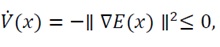
Integration into the generalized framework
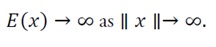
Figure 2 illustrates the transition from linear to nonlinear energy landscapes developed in this chapter for the nonlinear case, where quadratic nonlinearities are incorporated into the interaction functions A_i (x).
The proof begins with the generalized energy function:
 (44)
(44)
followed by the verification of the strictly positive definiteness of the Hessian matrix H(x) using Gershgorin’s Circle Theorem and the application of Condition 7, which constrains the nonlinear coefficients c_ik to preserve convexity and diagonal dominance.
These conditions jointly ensure the strict convexity of E(x) and the existence of a unique global minimum x_0. The introduction of the Lyapunov function V(x)=E(x)-E(x_0), together with LaSalle’s Invariance Principle, rigorously establishes that all trajectories in the state space monotonically converge to x_0. Thus, the logical progression of the proof demonstrates that even in systems governed by nonlinear interactions, both global stability and the spontaneous emergence of a unique stable structure are universally guaranteed through the principle of energy minimization.

Figure 2. Transition from linear to nonlinear energy landscapes. Comparison of linear (quadratic) and nonlinear potential surfaces. The diagram highlights how nonlinear self-interaction terms modify curvature and may generate local convex regions within a globally stable landscape.
Note 6: The restriction c_ij=0 for i≠jensures that all nonlinear contributions are self-interaction terms c_ii x_i^2, preserving the symmetry and diagonal dominance of the Hessian H(x). This diagonal structure prevents cross-coupled instabilities, allowing the Lyapunov and LaSalle analyses to remain valid globally. The resulting energy-minimizing equilibrium x_0 is thus guaranteed to be unique, stable, and physically interpretable as the self-organized configuration of the system.
4. Discussions
4.1 Interpretation of 'structure' in the context of ODE systems
In this study, the term “structure formation” refers to the spontaneous emergence and temporal persistence of a specific configuration of interacting state variables. Mathematically, this phenomenon corresponds to the convergence of the system’s dynamics toward a unique, globally stable equilibrium point—the energy minimum x_0 derived in Section 3.3. This equilibrium point represents a coherent onfiguration of all interacting components that remains robust against small perturbations and exhibits long-term stability under the system’s intrinsic dynamics. This interpretation of “structure” emphasizes the temporal stability of an organized state in the phase space, rather than its explicit spatial distribution or geometric form. In biological systems, such a structure could correspond to a differentiated cell phenotype haracterized by a stable gene-expression profile, or to a protein complex with fixed stoichiometry and conformation. In materials science, it may represent a thermodynamically stable crystalline phase or a particular molecular arrangement achieved through energetic relaxation. The key contribution of this theoretical framework lies in identifying the conditions under which such stable configurations emerge spontaneously from the intrinsic interactions of the system—without requiring external constraints or spatial coupling. While the present formulation does not directly address heterogeneous spatial distributions, it provides a foundational mechanism for local stability, which is a prerequisite for the formation of spatially organized patterns. Any self-organized spatial pattern, such as a Turing pattern or phase-separated domain, must be composed of stable local states that maintain internal equilibrium. Our framework rigorously defines how these stable local equilibria (x_0) arise from nonlinear interactions governed by the energy-minimization principle. Extending this ODE-based approach to spatially extended systems would involve introducing diffusive or advective transport terms, thereby transitioning from a temporal to a spatiotemporal framework. Our definition of “structure” as a stable equilibrium configuration of variables thus represents a mathematical abstraction of an organized state. Although the ODE system does not explicitly encode geometry or spatial gradients, the equilibrium x_0 can be interpreted as the local property or state that each element of a more complex physical or biological system tends to adopt. For example, in a population of interacting cells, x_0may represent a stable phenotypic attractor of an individual cell. When such cells interact through diffusion or signaling, these local attractors can collectively give rise to macroscopic spatial patterns. Therefore, omitting explicit spatial modeling at this stage is a deliberate theoretical choice—it allows for the establishment of the fundamental temporal stability mechanisms that underlie self-organization before introducing additional layers of spatial complexity. This framework thus provides a universal energetic foundation for understanding how systems composed of multiple interacting elements evolve toward stable, self-maintaining configurations.
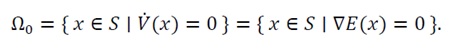
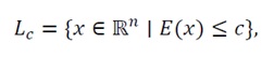
It serves as a versatile analytical tool that can later be extended to diverse physical contexts, such as morphogenesis, material self-assembly, or chemical pattern formation. Figure 3 schematically illustrates the assembly of a lipid bilayer under the proposed energy-minimization framework, demonstrating how local interactions spontaneously give rise to a globally stable configuration.
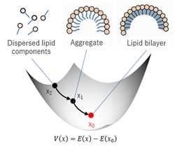
Figure 3. Multiscale coupling and hierarchical stability pathways.
The analysis developed in this study, based on an ordinary differential equation (ODE) framework, reveals how stable equilibrium configurations can spontaneously emerge through internal energy minimization. In this sense, a “structure” corresponds to a time-invariant configuration of interacting components—that is, a fixed point in state space determined by the system’s intrinsic nonlinear couplings.
This local stability is mathematically ensured by the strictly positive definiteness of the Hessian matrix H(x_0), which guarantees that any small perturbation around x_(0 ) decays over time. Although the present framework does not include explicit spatial derivatives or diffusion, its conclusions have profound implications for spatial pattern formation in extended systems described by reaction–diffusion equations (PDEs). In such systems, local dynamics (governed by ODE-like interactions) are coupled through spatial transport, giving rise to emergent macroscopic patterns. The stable equilibria identified in our ODE model correspond to the local steady states that individual “cells” or “units” may adopt within a larger spatial domain. The diagonal-dominance and strictly positive definiteness conditions established here thus ensure that each local unit remains stable while interacting diffusively with its neighbors—a necessary condition for the emergence of coherent spatial order. Future work will extend this framework to incorporate diffusion and stochasticity, thereby bridging the gap between temporal stability and spatial self-organization. Specifically, introducing diffusion terms into the gradient-flow system, ∂x/∂t=-∇E(x)+D∇^2 x, will enable investigation of how local minima x_0interact across space to form spatially heterogeneous steady states.
Similarly, incorporating stochastic perturbations within a stochastic differential equation (SDE) framework can clarify how noise influences the robustness and transition dynamics of these stable structures. Thus, the present deterministic ODE framework should be regarded as a foundational energetic model—a minimal yet rigorous description of self-stabilizing behavior. Its principles can be generalized to describe reaction–diffusion systems, pattern formation, and multiscale self-organization, where stable local equilibria form the elementary building blocks of spatially ordered phenomena. These directions represent promising avenues for future theoretical and computational research that aim to unify energetic stability, spatial coupling, and stochastic effects within a single comprehensive framework.
5. Theoretical Insights into the Emergence of Biological Structures
This chapter explores the practical and biological implications of the theoretical framework established in this study, which mathematically demonstrates how stable structures emerge in systems governed by multiple interacting forces. Building directly upon the results of Chapters 2 and 3, we extend the abstract theory of energy minimization and convex stability to a biological context—specifically, to the self-organization of membranes in oil–water systems and the formation of lipid bilayers, the fundamental structural basis of cell membranes. We aim to show that the principles of energy minimization, convexity, and global convergence toward a unique equilibrium x0  provide the universal mathematical foundation for these self-assembling biological systems.
5.1 The general nature of spontaneous structure formation
As rigorously derived in Chapters 2 and 3, systems governed by the gradient-flow dynamics x=-∇Ex,  converge toward a unique, globally stable equilibrium point x0
 when the Hessian matrix H(x)
 of the energy function E(x)
 is strictly positive definite and satisfies the diagonal-dominance condition (Condition 7). This convergence mechanism represents a universal principle of self-organization: the internal interactions among system components collectively generate an energy landscape whose minima correspond to stable, organized configurations. This insight captures a phenomenon widely observed across physics, chemistry, and biology—namely, that the nonlinear, collective interplay of individual components can autonomously produce ordered, predictable structures, transcending the simple summation of independent behaviors. The energy-gradient formulation thus provides a unifying explanation for why stable equilibrium configurations (or “structures”) emerge spontaneously without external control. The subsequent sections demonstrate how this general principle applies directly to membrane formation, one of the most fundamental examples of biological self-organization.
5.2 A Detailed theoretical interpretation for membrane-like structure formation: application to the lipid bilayer
The lipid bilayer represents the universal structural foundation of biological membranes, accounting for their selective permeability, flexibility, and self-healing properties essential for life [17,18]. From Overton’s early observations on lipid solubility [19], to Gorter and Grendel’s [20] experimental confirmation of a bilayer, and Stoeckenius’s electron microscopy revealing the trilaminar membrane [21], the spontaneous self-assembly of amphiphilic molecules into bilayers has been firmly established as a thermodynamic inevitability. This process is also recognized as a crucial step in the origin of protocells [22,23].
Our theoretical framework provides an abstract yet rigorous mathematical model to interpret this process as energy minimization and convergence to a unique stable equilibrium. Although the actual bilayer involves spatial and interfacial phenomena, our ODE formulation describes the thermodynamic compositional equilibrium that precedes and governs spatial organization.
5.2.1 Defining "structure" in the context of lipid bilayers
Within our framework, “structure” is defined as the unique stable equilibrium point x0 to which the system’s state vector x(t) converges under gradient dynamics. In the context of lipid assembly, x0 represents the stable compositional configuration achieved when the competing molecular forces—hydrophobic, electrostatic, and steric—reach dynamic equilibrium. This corresponds physically to the self-assembled lipid bilayer, with hydrophobic tails facing inward and hydrophilic heads exposed to the aqueous phase. Thus, the lipid bilayer exemplifies a stable attractor in the energy landscape, consistent with the mathematical results of Chapter 3.
5.2.2 Modeling the lipid bilayer as a stable energy minimum: mapping physical interactions to model parameters
To link physical interactions with the mathematical model, we define a simplified yet representative state vecto=(x1,x2)T, where
where
- x1
 : degree of lipid aggregation (fraction of monomers forming bilayer assemblies),
 - x2
 : degree of molecular alignment and orientation within the aggregated phase.
The system evolves according to x=-∇E(x), where E(x) represents the Gibbs free energy of the system.
For this case, we extend the general energy function introduced in Chapter 3 to include both self- and cross-nonlinear terms:
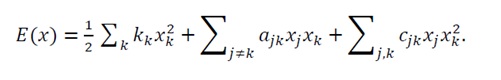 (45)
(45)
Unlike the analytically constrained form in Chapter 3 (where only cii≠0 ), here cjk
 terms (with j≠k
 ) are conceptually included to capture cooperative nonlinearities—a realistic feature of lipid aggregation.
The coefficients in Eq.(45) correspond to distinct physical effects:
- kk
 : self-interaction coefficients (intrinsic stiffness), penalizing deviations from equilibrium;
 - ajk
 : linear cross-couplings (hydrophobic and interfacial interactions) that drive aggregation and molecular orientation;
 - cii
 : nonlinear cooperative terms accounting for concentration thresholds (e.g., critical micelle concentration) and steric repulsion at high packing density.
Minimization of E(x) leads the system to a thermodynamically optimal state x0 , in which aggregation and alignment reach a stable balance—corresponding to a stable bilayer configuration.
Footnote:
Note 7: For clarity, all nonlinear coefficients are denoted cii , representing self-nonlinearity. When needed for general index expressions, one may equivalently write cik with the convention cik=0
 for i≠k
 . This maintains full consistency with the assumption introduced in Chapter 3.
5.2.3 Mathematical proof of structural stability: The lipid bilayer as a "structure"
The spontaneous formation of lipid bilayers provides a representative example of how the proposed energy?minimization framework explains the emergence of stable structures in multi?component physical systems. In aqueous environments, amphiphilic molecules, such as phospholipids, self?assemble into bilayer membranes without external control. This process can be interpreted as a natural relaxation toward a global energy minimum, where hydrophobic interactions, van der Waals forces, and entropic effects collectively determine the final equilibrium configuration. The proposed energy?minimization model describes this self?assembly as the descent of a dynamical system governed by an energy function E(x) , where each variable xi represents a structural degree of freedom such as molecular orientation, local packing density, or surface curvature. When the total energy function E(x) is minimized, all intermolecular forces—including hydrophobic, electrostatic, and entropic contributions—reach a balanced configuration that corresponds to a stable bilayer state. This equilibrium point x0 defines a unique compositional configuration in which the molecular system attains its lowest possible energy under the given physical constraints. Within the parameter range where the uniform strong convexity assumption (U) holds, the energy landscape remains globally convex, guaranteeing the uniqueness of this equilibrium. This restriction clarifies that the uniqueness claim applies only within the convex regime, consistent with the model’s physical validity range. Outside this regime, where the curvature of E(x) may lose uniform positivity, multiple metastable configurations can emerge—corresponding, for example, to micelles or vesicular intermediates. Thus, the strong convexity assumption delineates the thermodynamic range within which the bilayer structure remains the unique global minimizer of the system’s free energy. Under these conditions, the gradient flow dynamics x=-∇E(x)
 guarantee monotonic convergence toward x0 . The Lyapunov function V(x)=E(x)-E(x0)
  decreases strictly along all trajectories, confirming asymptotic stability. Physically, this means that small perturbations to the bilayer—such as local fluctuations in lipid orientation or molecular displacement—will relax spontaneously back to the equilibrium configuration, restoring the structural integrity of the membrane. This theoretical perspective reproduces the experimentally observed stability of lipid bilayers, where once formed, membranes exhibit high resilience to thermal and mechanical disturbances. The bilayer thus represents a self?organized structure emerging from the intrinsic minimization of total system energy, requiring no external control. In this way, the model provides a rigorous mathematical foundation for understanding how spontaneous structural stabilization arises from the coupled interactions among molecular components, unifying thermodynamic intuition with dynamical?systems theory.
5.2.4 The lipid bilayer as a "structure" defined by this theory
From the above analysis, three key conclusions follow:
1. Definition of the bilayer as a structure
The lipid bilayer corresponds to the stable equilibrium x0 of the system, representing the spontaneous organization of amphiphilic molecules into a minimal-energy configuration. This equilibrium is not merely a metastable aggregate but a provably stable structure arising from the convexity of E(x) .
2. Driving forces of formation
The bilayer emerges from the interplay of hydrophobic attraction, interfacial tension minimization, and steric repulsion.
These forces collectively act to minimize E(x) , leading to autonomous self-assembly—a process that can be regarded as thermodynamically inevitable under the given physical constraints.
3. Mathematical guarantee of stability
The equilibrium x0 satisfies both ∇E(x0)=0
 and H(x0)?0
 .
.
By Condition 7, the convexity is preserved even under nonlinear perturbations cjk , ensuring robustness against fluctuations. This provides a rigorous mathematical basis for the stability and persistence of lipid membranes, as observed empirically in biological and prebiotic systems.
5.3 Limitations and future directions
While the proposed ODE-based framework provides a universal foundation for the temporal convergence of interacting systems to stable configurations, it does not explicitly describe spatial structure or thermal noise.
However, these limitations define clear and fertile directions for future work:
- Spatial Extension (ODE → PDE): By integrating diffusion or advection terms into the energy-gradient formulation, ∂x∂t=-∇E(x)+D∇2x,
 the model can be extended to describe reaction–diffusion or phase-field systems, bridging temporal and spatial self-organization.
 - Higher-order nonlinearities: Introducing cubic or threshold-type nonlinearities can capture multistability and oscillatory dynamics, extending the model to phenomena such as excitable media or biochemical oscillations.
- Anisotropy and geometric constraints: Incorporating direction-dependent interactions and boundary conditions will allow the model to represent membrane curvature, domain formation, and morphogenetic growth.
- Stochastic extensions: Expanding to stochastic differential equations (SDEs) can quantify the role of noise, molecular discreteness, and thermal fluctuations in initiating or stabilizing self-assembly. These extensions build directly upon the convexity and Lyapunov stability conditions derived in Chapter 3, translating temporal stability into spatial and stochastic domains. Through such developments, the framework may evolve into a comprehensive mathematical theory of self-organization, capable of explaining and predicting structure formation across physical, chemical, and biological systems.
5.4 Implications for neural morphogenesis and patterning
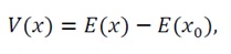
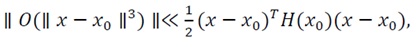
Figure 4 illustrates, across three conceptual panels, how neuronal morphogenesis can be interpreted as the descent of a dynamical system along an energy landscape shaped by multiple competing cues. In panel A, an axon extends from the neuronal soma within a field of attractive (blue) and repulsive (red) guidance signals. These cues define an effective potential landscape E(x):  attractants form valleys that lower local energy, whereas repellents create hills that raise it. In panel B, the growth cone follows the composite gradient of this potential, performing a local energetic descent toward the minimum point x0 . As derived in Eqs. (34)–(39) of Chapter 3, the Lyapunov function V(x)=E(x)-E(x0)
 decreases monotonically over time (V(x)=-?∇E(x)?2≤0),
 guaranteeing convergence to this stable configuration. In panel C, a balance between attractive and repulsive forces yields a self-organized neural architecture characterized by stable axonal trajectories, dendritic arborization, and coherent spatial patterning. Together, these panels provide a physical–morphogenetic interpretation of neural development: neural connectivity arises spontaneously—without centralized control—from the minimization of energy under multiple interacting constraints. This mirrors the broader thermodynamic principle that biological systems evolve by minimizing free energy to attain stable internal states, as articulated in Friston’s Free Energy Principle [24]. While Friston’s “free energy” refers to an informational variational quantity, the present energy E(x) represents a physical potential governing morphogenetic dynamics; both share the same descent mechanism but differ in domain and scale. The energetic-minimization framework developed in this study thus provides a unified theoretical foundation for understanding not only physical and chemical self-organization but also the spontaneous emergence of neural architecture—where pattern and connectivity naturally arise from energy-constrained dynamics. Hence, the same minimization principle that explains molecular self-assembly (Section 5.2) also extends hierarchically to neuronal morphogenesis, suggesting a universal energetic law governing biological structure formation across scales. The energetic-minimization principle offers a consistent explanation for neural morphogenesis—from axon guidance to network-level patterning—within the same mathematical framework.
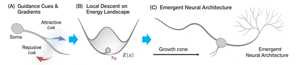
Figure 4. Application to spontaneous structure formation in complex systems. Representative examples of emergent structures (e.g., lipid bilayer formation or pattern self-organization) interpreted through the proposed energy-minimization framework. Each configuration corresponds to a stable equilibrium on the derived energy surface.
Classical observations by Ramón y Cajal [25] established that neuronal morphology reflects both intrinsic growth tendencies and environmental constraints. Later, Goodhill [26] formalized these processes using diffusion-based guidance fields, and van Ooyen [27] extended them to network dynamics, showing that collective neuronal growth can be modeled as energy-based optimization. Each growth cone, responding to local gradients of attractants and repellents, effectively performs a gradient descent along a multidimensional energy surface, converging to a stable equilibrium architecture x0 . A striking parallel thus emerges between this morphogenetic framework and Friston’s variational free-energy theory: both describe systems that evolve by reducing energetic or informational uncertainty, converging toward self-consistent, stable configurations. The present framework, however, grounds this principle in physical morphogenesis, showing that even at subcellular scales, energy minimization alone can generate ordered neural structures. In summary, neural development and patterning emerge naturally—as physical realizations of energy minimization under multiple interacting constraints—unifying molecular, cellular, and cognitive levels of organization within a single theoretical landscape.
Conclusion
This study has established a rigorous theoretical framework for the spontaneous formation of stable structures in nonlinear systems through the principle of energy minimization. Building upon the linear model introduced in Chapter 2, the framework was extended to include quadratic nonlinearities of the form ciixi2 , while preserving analytical tractability and physical interpretability. The resulting nonlinear energy function E(x) was demonstrated to possess a unique global minimum x0 , toward which all trajectories converge asymptotically under gradient-flow dynamics. Through systematic derivations in Sections 3.2–3.3, it was shown that the Hessian matrix H(x)=∇2E(x)
 remains strictly positive definite when the nonlinear coefficients cii
 satisfy the diagonal-dominance constraint (Condition 7). This guarantees the strict convexity of the energy function and thereby ensures the local strong convexity of E(x) in the neighborhood of x0 . Under additional assumptions of Uniform Strong Convexity (U) and Coercivity (C), the convexity extends globally, proving that E(x) admits a unique global minimizer. By defining the Lyapunov function V(x)=E(x)-E(x0) , it was proven (Sections 3.3.1–3.3.3) that V(x)
 is strictly positive definite and that its time derivative satisfies V(x)≤0
 . Applying LaSalle’s Invariance Principle, every trajectory governed by the gradient-flow system x=-∇E(x)
 converges to the invariant set where ∇E(x)=0
 , which—due to the strong convexity of E(x) —consists solely of the equilibrium point x0 . Thus, the system exhibits global asymptotic stability, with all trajectories monotonically approaching the unique energy-minimizing configuration. The influence of the nonlinear terms ciixi2 was further analyzed in the section Influence and Stability of Non-Linear Terms.
A Taylor expansion around the equilibrium point x0 revealed that these nonlinearities contribute only to higher-order terms O(?x-x0?3) , which remain bounded within the convex energy landscape. When the coefficients cii
  satisfy Condition 7, these higher-order corrections are small enough not to alter the positive curvature governed by the quadratic term, ensuring that convexity and convergence are preserved. This bounded nonlinearity framework, as discussed in Influence and Stability of Non-Linear Terms, quantitatively explains how moderate nonlinear effects can coexist with global stability—enabling complex yet self-organizing behavior without compromising the uniqueness of the equilibrium. In summary, this work provides a unified and mathematically rigorous proof that:
- Energy minimization governs the spontaneous stabilization of nonlinear systems;
- Diagonal dominance and self-nonlinearity bounds ensure the convexity of the energy landscape; and
- Lyapunov stability and LaSalle’s invariance guarantee convergence toward the unique global equilibrium.
These findings bridge local convexity analysis and global convergence theory, demonstrating that even in the presence of nonlinear self-interactions, a system governed by energy minimization inevitably evolves toward a single, stable, self-organized structure.
References
2. Gierer A, Meinhardt H. A theory of biological pattern formation. Kybernetik. 1972;12(1):30–9.
3. Oster GF, Murray JD. Pattern formation models and developmental constraints. J Exp Zool. 1989 Aug;251(2):186–202.
4. Kondo S, Miura T. Reaction-diffusion model as a framework for understanding biological pattern formation. Science. 2010 Sep 24;329(5999):1616–20.
5. Yamaguchi M, Yoshimoto E, Kondo S. Pattern regulation in the stripe of zebrafish suggests an underlying dynamic and autonomous mechanism. Proc Natl Acad Sci U S A. 2007 Mar 20;104(12):4790-3.
6. Nakamasu A, Takahashi G, Kanbe A, Kondo S. Interactions between zebrafish pigment cells responsible for the generation of Turing patterns. Proc Natl Acad Sci U S A. 2009 May 26;106(21):8429-34.
7. Hao Y, Huang H, Jia Z, Zhou Y, Zhang H. Complex pattern transitions and multistable states in a reaction-diffusion system with non-uniform domain. Communications in Nonlinear Science and Numerical Simulation. 2020;89:105282.
8. Kondo S, Iwasaki T. Fish skin patterns as a living Turing wave. Nature. 2021;576(7785):771–5.
9. Kicheva A, Pantazis P, Bollenbach T, Kalaidzidis Y, Bittig T, Jülicher F, et al. Kinetics of morphogen gradient formation. Science. 2007 Jan 26;315(5811):521–5.
10. Wartlick O, Kicheva A, González-Gaitán M. Morphogen gradient formation. Cold Spring Harbor Perspectives in Biology. 2009;1(3):a001255.
11. Green JB, Sharpe J. Positional information and reaction-diffusion: two big ideas in developmental biology combine. Development. 2015 Apr 1;142(7):1203–11.
12. Gerschgorin S. Über die Abgrenzung der Eigenwerte einer Matrix. Izv. Akad. Nauk. USSR Otd. Fiz.-Mat. Nauk. 1931;7:749–54.
13. LaSalle J. Some extensions of Liapunov's second method. IRE Transactions on circuit theory. 1960 Dec;7(4):520–7.
14. Boyd S, Vandenberghe L. Convex Optimization. Cambridge: Cambridge University Press; 2004
15. Khalil HK. Nonlinear Systems. Upper Saddle River: Prentice Hall; 2002.
16. Horn RA, Johnson CR. Matrix Analysis. 2nd ed. Cambridge: Cambridge University Press; 2012.
17. Singer SJ, Nicolson GL. The fluid mosaic model of the structure of cell membranes. Science. 1972 Feb 18;175(4023):720–31.
18. Alberts B, Johnson A, Lewis J, Raff M, Roberts K, Walter P. Molecular biology of the cell. 4th ed. New York: Garland Science; 2002.
19. Overton E. Ueber die allgemeinen osmotischen Eigenschaften der Zelle. Vierteljahrschr Naturf Ges Zurich. 1899;44:88–135.
20. Gorter E, Grendel F. On Bimolecular Layers of Lipoids on the Chromocytes of the Blood. J Exp Med. 1925 Mar 31;41(4):439–43.
21. Stoeckenius W. The molecular structure of lipid-water systems and cell membrane models studied with the electron microscope. Journal of Cell Biology. 196212(2):221–9.
22. Deamer DW. The first living systems: a bioenergetic perspective. Microbiol Mol Biol Rev. 1997 Jun;61(2):239–61.
23. Luisi PL. The Emergence of Life: From Chemical Origins to Synthetic Cells. Cambridge: Cambridge University Press; 2006.
24. Friston K. The free-energy principle: a unified brain theory? Nat Rev Neurosci. 2010 Feb;11(2):127–38.
25. Cajal SR. Histology of the Nervous System of Man and Vertebrates. Oxford: Oxford University Press; 1911
26. Goodhill GJ. Mathematical guidance models for axon growth. Journal of Theoretical Biology. 1998;194(4):405–10.
27. van Ooyen A. Using theoretical models to analyse neural development. Nat Rev Neurosci. 2011 Jun;12(6):311–26.